Steerable filters - image gradients (based AI studio)

AI studio default settings

# 查看当前挂载的数据集目录, 该目录下的变更重启环境后会自动还原
# View dataset directory. 
# This directory will be recovered automatically after resetting environment. 
!ls /home/aistudio/data
!python --version

# 查看工作区文件，该目录下除data目录外的变更将会持久保存。请及时清理不必要的文件，避免加载过慢。
# View personal work directory. 
# All changes, except /data, under this directory will be kept even after reset. 
# Please clean unnecessary files in time to speed up environment loading. 
!ls /home/aistudio

# 查看当前的python包
!pip list

# 如果需要进行持久化安装, 需要使用持久化路径, 如下方代码示例:
# If a persistence installation is required, 
# you need to use the persistence path as the following: 
!mkdir /home/aistudio/external-libraries
!pip install beautifulsoup4

# 同时添加如下代码, 这样每次环境(kernel)启动的时候只要运行下方代码即可: 
# Also add the following code, 
# so that every time the environment (kernel) starts, 
# just run the following code: 
import sys 
sys.path.append('/home/aistudio/external-libraries')

Steerable filter (Sobel Kernels)

Generate the test images

import numpy as np
import cv2
from matplotlib import pyplot as plt

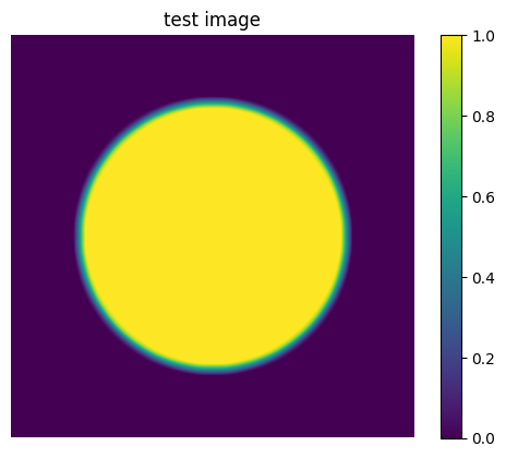
# size of test image
n = 512

# get test image of a circle
test_image = np.zeros((n, n))
cv2.circle(test_image, center=(n//2, n//2), radius=n//3, color=(255,), thickness=-1)

# blurring the image
cv2.GaussianBlur(test_image, ksize=(15, 15), sigmaX=13, dst=test_image)

# 0-1 normalize
test_image = cv2.normalize(test_image, dst=None, alpha=0, beta=1, norm_type=cv2.NORM_MINMAX, dtype=cv2.CV_32FC1)

# show image
plt.imshow(test_image)
plt.axis('off')  # 不显示坐标轴
plt.title('test image')
plt.colorbar()
plt.show()

Creat the kernel

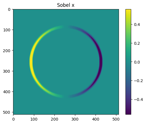
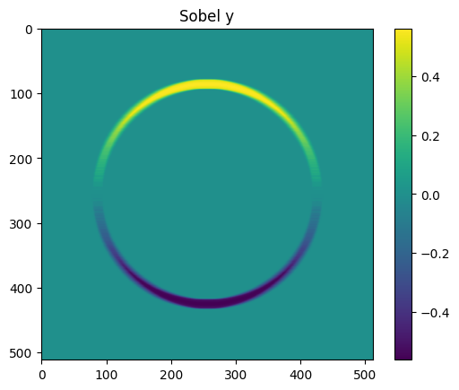
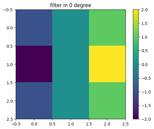
# Sobel kernels
# 0 degree： direction: right
G_x = np.array([[-1, 0, 1], 
                [-2, 0, 2], 
                [-1, 0, 1]])
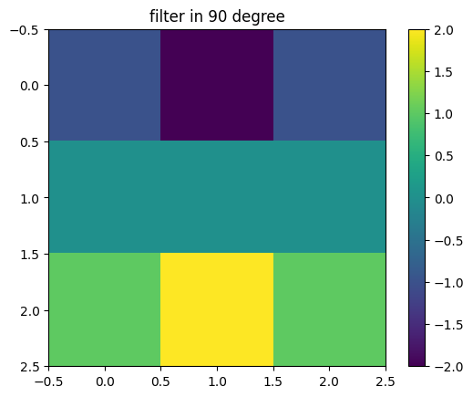
# 90 degree： direction: down
G_y = np.array([[-1, -2, -1], 
                [0,   0,  0], 
                [1,  2,  1]])
                
# apply the filter
# ddepth=-1 表示输出图像与输入图像具有相同的深度
test_image_x = cv2.filter2D(src=test_image, ddepth=-1, kernel=G_x)
test_image_y = cv2.filter2D(src=test_image, ddepth=-1, kernel=G_y)

# show image
plt.imshow(test_image_x)
plt.title('Sobel x')
plt.colorbar()
plt.show()


plt.imshow(test_image_y)
plt.title('Sobel y')
plt.colorbar()
plt.show()

Creat filter

Two kernels are already created. One oriented at 0 degree, one oriented at 90 degree, they are denoted as $G^0$ and $G^{90}$, respectively.

The responses of these two kernels are recorded as $R^0$ and $R^{90}$, respectively.

We can steer the gradient direction by taking a linear combination of these responses:

\[R^{\theta} = cos(\theta)R^0 + sin(\theta)R^{90}\]

where, for the image $I(x,y)$

\[R^0 = I(x,y) * G^0\] \[R^{90} = I(x,y) * G^{90}\]

we can rewrite the equation to get the unique filter using the distribute property of convolution,

\[R^{\theta} = cos(\theta)R^0 + sin(\theta)R^{90}\] \[R^{\theta} = cos(\theta)(I(x,y) * G^0) + sin(\theta)(I(x,y) * G^{90})\] \[R^{\theta} = I(x,y)*(cos(\theta)G^0 + sin(\theta)G^{90})\]

Hence, $ G^{\theta} = cos(\theta)G^0 + sin(\theta)G^{90} $

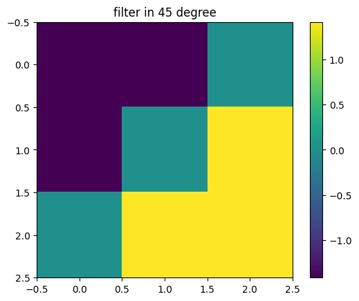
# creat steerable filter
theta = np.radians(45)
G_theta = np.cos(theta)*G_x + np.sin(theta)*G_y

plt.imshow(G_x)
plt.title('filter in 0 degree')
plt.colorbar()
plt.show()

plt.imshow(G_y)
plt.title('filter in 90 degree')
plt.colorbar()
plt.show()


plt.imshow(G_theta)
plt.title('filter in 45 degree')
plt.colorbar()
plt.show()

Filters kernels

Considering the gasussian shape function, given by,

$G = e^{-(x^2+y^2)}$

Design the filters by taking the first derivative of a Gaussian funtion:

$ G^0 = \frac{\partial}{\partial{x}} e^{-(x^2+y^2)} = 2xG $

$ G^{90} = \frac{\partial}{\partial{y}} e^{-(x^2+y^2)} = -2yG $

# define the function: Gaussian Function
G = lambda x, y: np.exp(-(x**2 + y**2))
G0 = lambda x, y: 2*x*G(x, y)
G90 = lambda x, y: 2*y*G(x, y)

# define the index of kernel
x_index = np.array([[-1, 0, 1], 
                    [-1, 0, 1], 
                    [-1, 0, 1]])
y_index = np.array([[-1, -1, -1], 
                    [0,  0, 0], 
                    [1, 1, 1]])

# gaussian kernel
gk = G(x_index, y_index);
gk0 = G0(x_index, y_index);
gk90 = G90(x_index, y_index);
print(gk)
print(gk0)
print(gk90)

gk_theta = np.cos(theta)*gk0 + np.sin(theta)*gk90
R_gk0 = cv2.filter2D(src=test_image, ddepth=-1, kernel=gk0)
R_gk90 = cv2.filter2D(src=test_image, ddepth=-1, kernel=gk90)
R_gktheta = cv2.filter2D(src=test_image, ddepth=-1, kernel=gk_theta)

plt.imshow(gk0)
plt.title('filter in 0 degree')
plt.colorbar()
plt.show()

plt.imshow(gk90)
plt.title('filter in 90 degree')
plt.colorbar()
plt.show()


plt.imshow(gk_theta)
plt.title('filter in 45 degree')
plt.colorbar()
plt.show()

plt.imshow(R_gk0)
plt.title('filtered image in 0 degree')
plt.colorbar()
plt.show()

plt.imshow(R_gk90)
plt.title('filtered image in 90 degree')
plt.colorbar()
plt.show()

plt.imshow(R_gktheta)
plt.title('filtered image in 45 degree')
plt.colorbar()
plt.show()

[[0.13533528 0.36787944 0.13533528]
 [0.36787944 1.         0.36787944]
 [0.13533528 0.36787944 0.13533528]]
[[-0.27067057  0.          0.27067057]
 [-0.73575888  0.          0.73575888]
 [-0.27067057  0.          0.27067057]]
[[-0.27067057 -0.73575888 -0.27067057]
 [ 0.          0.          0.        ]
 [ 0.27067057  0.73575888  0.27067057]]