Zero padding FFT
Fast Fourier Transform (FFT) is an essential too for analyzing a signal's frequency content. One common operation before applying FFT is zero-padding, appending zeros to the end of a signal to increase the total number of samples used in the transform.
Zero-padding
Zero-padding refers to adding extra zero-valued smaples to the time domain signal before performing the FFT.
The benefits
Increase the number of FFT Bins (Spectral Interpolation)
Zero-padding increases the number of frequency points in the FFT output, effectively interpolating the original FFT bins. This operation does not add new frequency information, but it:
- interpolate the existing spectrum.
- make the spectrum look smoother and more continuous.
- helps locate peaks more precisely.
Think of it like enlarging a digital photo, we can not get more detail, but we get a clearer view of what's already there.
Zero-Padded FFT-Based Convolution
In FFT-based convolution, zero-padding is required to prevent time-domain aliasing. When convolving two signals of length
𝑁 and 𝑀, the FFT length must be at least 𝑁+𝑀−1.
What Zero-Padding Does Not Do
Does Not Improve Frequency Resolution
While zero-padding increases the number of FFT bins, it does not improve the frequency resolution in the physical sense. The frequency resolution depends on the duration of the signal:
$ \Delta f=\frac{1}{T} $
where, $ T $ is the time span of the original signal.
Zero-padding cannot overcome the limitations imposed by a short time window.
It’s important to understand that all the additional points are derived through mathematical interpolation — no new data is being introduced.
Example
Set Up Sampling Parameter and Frequencies
1
2
3
fs = 1000;          % Sampling rate (samples per second, or Hz)
f1 = 50; f2 = 52;   % Two sine wave frequencies close to each other
amp = 1;            % Amplitude of the sine waves
- Two closely spaced frequencies: 50 Hz and 52 Hz.
- Sampling rate is 1000 Hz.
Generate a Short-Duration Signal (0.2 seconds)
1
2
3
T1 = 0.2;
t1 = 0:1/fs:T1-1/fs;
x1 = amp*sin(2*pi*f1*t1) + amp*sin(2*pi*f2*t1);
This creates a short signal that lasts 0.2 seconds.
The signal $ x_1 $ is a sum of the two sine waves (50 Hz and 52 Hz).
Frequency resolution is: $ \Delta f = \frac{1}{0.2 S} = 5 Hz $
Generate a Long-Duration Signal (2 seconds)
1
2
3
T2 = 2;
t2 = 0:1/fs:T2-1/fs;
x2 = amp*sin(2*pi*f1*t2) + amp*sin(2*pi*f2*t2);
- This creates a longer signal lasting 2 seconds.
- Frequency resolution improves to: $ \Delta f = \frac{1}{2 S} = 0.5 Hz $
- This higher resolution allows us to separate the two close frequencies.
Compute FFT with Zero-Padding
1
2
3
X1 = fft(x1, 4096);
X2 = fft(x2, 4096);
f = (0:4095)*(fs/4096);  % Frequency axis
- Both signals are zero-padded to 4096 points before computing FFT.
- This increases the number of frequency bins, but does not change the actual resolution.
Plot the Spectra
1
2
3
4
5
6
7
8
9
figure
subplot(2,1,1);
plot(f, abs(X1), "LineWidth", 2); xlim([40 60]);
title("Short signal (0.2s) — Resolution = 5 Hz");
set(gca,"FontSize",15, "FontName","Times New Roman");
subplot(2,1,2);
plot(f, abs(X2), "LineWidth", 2); xlim([40 60]);
title("Long signal (2s) — Resolution = 0.5 Hz");
set(gca,"FontSize",15, "FontName","Times New Roman");
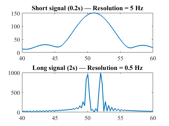
- The top subplot shows the FFT of the short signal — the two sine waves are not clearly separated.
- The bottom subplot shows the FFT of the long signal — the two sine waves appear as two distinct peaks.